Exploring scikit-learn
Introduction
For my current NEAT project, I read the paper A Comparative Study of Supervised Machine Learning Algorithms for Stock Market Trend Prediction to learn how others approached stock market prediction using supervised machine learning algorithms. This paper compared the accuracy between Support Vector Machine, Random Forest, K-Nearest Neighbor, Naive Bayes, and SoftMax algorithms. After reading about these different algorithms, I took it upon myself to learn more about the scikit-learn python library. I am learning how to use scikit-learn because it will give me the ability to implement some the algorithms outlined in the paper. The algorithms I have covered so far include:
• Random Forest
• K-Nearest Neighbors
• Support Vector Machine
Random Forest
The first algorithm I sought to better understand was the Random Forest algorithm. This algorithm is made up of multiple decision trees. A decision tree learns simple decision rules from the data and produces a output. Each tree is used on a different sub sample of the dataset and averaging is used to improve accuracy. The decision trees all “vote” by producing outputs, and whatever the most popular output is becomes the algorithms output.
I first imported my data as a Pandas data frame and split it up into a training section and a testing section. I then created a Random Forest algorithm using the scikit-learn random forest classifier. After running the algorithm a few times, I noticed that the accuracy was unusually high. After some investigation, I discovered that the algorithms were predicting the stock price movement for the current day instead of one day in the future. After fixing the problem, the accuracy on the testing dataset stayed around 50%. Here is the code that I wrote:
1
2
3
4
5
6
7
8
9
10
11
12
13
14
15
16
17
18
19
20
21
22
23
24
25
26
27
28
29
30
31
32
33
34
35
36
37
38
 import csv
import pandas as pd
from sklearn.model_selection import train_test_split
from sklearn.ensemble import RandomForestClassifier
from sklearn import metrics
from sklearn.metrics import classification_report

#this opens the file and puts the data in a pandas dataframe
data = pd.read_csv('RandomForest.csv')
data.head()

#setting the size of the training dataset
training_size = .7
split = int(len(data)*.7)

#Identifying all of the inputs and the expected output
X=data[['Open','High','Low','Close','Volume','Accumulation Distribution Line','MACD','Chaikan Oscillator (CHO)','Highest closing price (5 days)',
'Lowest closing price (days)','Stochastic %K (5 days)','%D','Volume Price Trend (VPT)','Williams %R (14 days)','Relative Strength Index','Momentum (10 days)',
'Price rate of change (PROC)','Volume rate of change (VROC)','On Balance Volume (OBV)']]
y=data['Outputs']

#splitting the dataframe into a training and testing dataset
X_train = X[:split]
X_test = X[split:]
y_train = y[:split]
y_test = y[split:]

#create a the random forest with 500 decision trees
clf=RandomForestClassifier(n_estimators=500)

#train the model on the training data
clf.fit(X_train,y_train)

#making predictions on the testing data
y_pred=clf.predict(X_test)

#printing the testing accuracy
print("Accuracy:",metrics.accuracy_score(y_test, y_pred))
K-Nearest Neighbors
The next algorithm I studied was the K-Nearest Neighbors algorithm. The nearest neighbor method looks for the most similar trading days. The predefined number of the most similar trading days become the nearest neighbors. Just like the decision trees in the Random Forest algorithm, the nearest neighbors “vote”. Instead of using decision trees to produce an output, the K-Nearest Neighbor algorithm uses the actual expected output for the most similar trading days. The most popular output becomes of the neighbors becomes the algorithms output. If 5 of the nearest neighbors had the closing stock price go up and 3 neighbors had the stock price go down, the prediction will be that the stock price goes up.
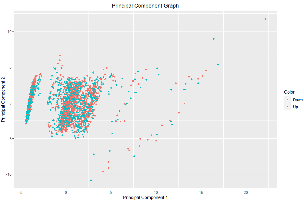
While studying this algorithm, I learned that K-Nearest Neighbor algorithms performs better with a lower number of features/inputs. To reduce the size of my dataset, I first normalized it with the standard scaler tool from scikit-learn. I then used PCA to shrink the number of inputs in my dataset down to two while preserving the variance in the dataset. Here is my K-Nearest Neighbors code:
1
2
3
4
5
6
7
8
9
10
11
12
13
14
15
16
17
18
19
20
21
22
23
24
25
26
27
28
29
30
31
32
33
34
35
36
37
38
39
40
41
42
43
44
45
 import csv
import pandas as pd
from sklearn import metrics
from sklearn.metrics import classification_report
from sklearn.neighbors import KNeighborsClassifier
from sklearn.decomposition import PCA
from sklearn.preprocessing import StandardScaler

#this opens the CSV File
data = pd.read_csv('RandomForest.csv')
data.head()

#preprocessing and normalizing
Features = ['Open','High','Low','Close','Volume','Accumulation Distribution Line','MACD','Chaikan Oscillator (CHO)','Highest closing price (5 days)',
'Lowest closing price (days)','Stochastic %K (5 days)','%D','Volume Price Trend (VPT)','Williams %R (14 days)','Relative Strength Index','Momentum (10 days)',
'Price rate of change (PROC)','Volume rate of change (VROC)','On Balance Volume (OBV)']

X = data.loc[:, Features].values
Y = data.loc[:,['Outputs']].values

#normalizing the dataset
X = StandardScaler().fit_transform(X)

#performing PCA
PCA = PCA(n_components=2)
Components = PCA.fit_transform(X)
ComponentDf = pd.DataFrame(data=Components)

#setting the size of the training set
training_size = .8
split = int(len(data)*training_size)

#splitting up the dataset
X_train = pd.DataFrame(data=ComponentDf[:split])
X_test = pd.DataFrame(data=ComponentDf[split:])
Y_train = pd.DataFrame(data=Y[:split])
Y_test = pd.DataFrame(data=Y[split:])

#create the K Nearest Neighbor Algorithm and running the algorithm
clf=KNeighborsClassifier(n_neighbors=5)
clf.fit(X_train, Y_train.values.ravel())
Y_pred=clf.predict(X_test)

#printing the testing accuracy
print("Accuracy:",metrics.accuracy_score(Y_test, Y_pred))
After performing principal component analysis on my dataset, I graphed the principal components to better understand the data. After creating the graph, it became clear why the accuracy of my K-Nearest Neighbor algorithm stayed around 50%. Both expected outputs (Stock price going up or down) are clustered together.
Support Vector Machine
A Support Vector Machine is a machine learning tool that uses a hyperplane to define data points. Instead of looking at the nearest neighbors like a KNN, I like to think that Support Vector Machines split up data points into different neighborhoods. For example, if we use the two components from my PCA analysis, a SVM will create a one dimensional hyperplane splitting up the data into two “neighborhoods”. The hyperplane will create decision boundaries that maximize the margins from both expected outputs. The graph below shows the data points and the decision boundaries created by my SVM.
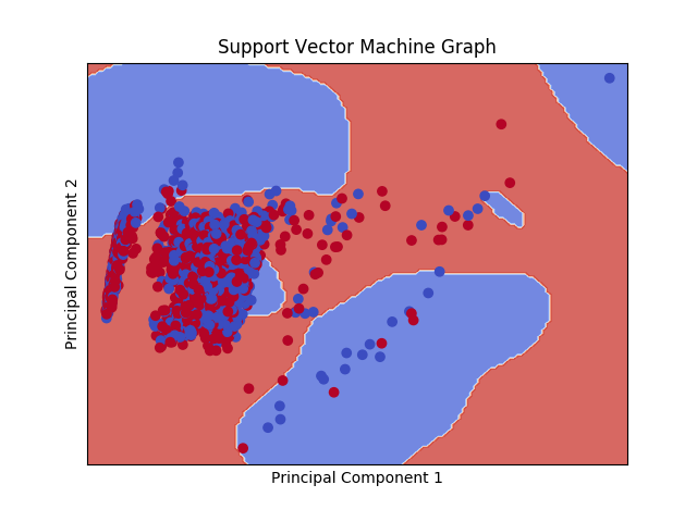
Any data point that falls into the blue background gets categorized as a 0 (closing stock price goes down). To create this graph, I used a Support Vector Machine with a RBF kernel. Kernel functions allow SVMs to create hyperplanes in high dimensional data without having to calculate the coordinates of the data in that space. Here is my Support Vector Machine Code:
1
2
3
4
5
6
7
8
9
10
11
12
13
14
15
16
17
18
19
20
21
22
23
24
25
26
27
28
29
30
31
32
33
34
35
36
37
38
39
40
41
42
43
44
45
46
47
48
49
50
51
52
53
54
55
56
57
58
59
60
61
62
63
64
65
66
67
68
69
70
71
72
73
74
75
76
77
78
79
80
81
82
83
84
85
86
87
 #support vector machine

import csv
import pandas as pd
from sklearn import metrics
from sklearn.metrics import classification_report
from sklearn import svm
from sklearn.decomposition import PCA
from sklearn.preprocessing import StandardScaler
import matplotlib.pyplot as plt
import numpy as np

#this opens the CSV File
data = pd.read_csv('RandomForest.csv')
data.head()

#setting the size of the training dataset
training_size = .7
split = int(len(data)*.7)

#Identifying all of the inputs and the expected output
X=data[['Open','High','Low','Close','Volume','Accumulation Distribution Line','MACD','Chaikan Oscillator (CHO)','Highest closing price (5 days)',
'Lowest closing price (days)','Stochastic %K (5 days)','%D','Volume Price Trend (VPT)','Williams %R (14 days)','Relative Strength Index','Momentum (10 days)',
'Price rate of change (PROC)','Volume rate of change (VROC)','On Balance Volume (OBV)']]
y=data['Outputs']

#splitting the dataframe into a training and testing dataset
X_train = X[:split]
X_test = X[split:]
y_train = y[:split]
y_test = y[split:]

#create the support vector machine
svc = svm.SVC(kernel='rbf', C=1.0)
svc.fit(X_train, y_train)
y_pred = svc.predict(X_test)

#printing the testing accuracy
print("Accuracy:",metrics.accuracy_score(y_test, y_pred))

##################################################
#The next section transforms the dataset#
#And graphs the components with decision boundries

#Normalizing the dataset
X = StandardScaler().fit_transform(X)

#performing PCA
PCA = PCA(n_components=2)
Components = PCA.fit_transform(X)
ComponentDf = pd.DataFrame(data=Components,columns = ['principal component 1', 'principal component 2'])

#transforming the dataset
X = ComponentDf.to_numpy()
y = y.ravel()

h = 0.2

# create a mesh to plot in
x_min, x_max = X[:, 0].min() - 1, X[:, 0].max() + 1
y_min, y_max = X[:, 1].min() - 1, X[:, 1].max() + 1
xx, yy = np.meshgrid(np.arange(x_min, x_max, h),
                     np.arange(y_min, y_max, h))

#create the support vector machine
svc = svm.SVC(kernel='rbf', C=1.0).fit(X, y)

#graphing the data
Z = svc.predict(np.c_[xx.ravel(), yy.ravel()])

# Put the result into a color plot
Z = Z.reshape(xx.shape)
plt.contourf(xx, yy, Z, cmap=plt.cm.coolwarm, alpha=0.8)

# Creating the plot
plt.scatter(X[:, 0], X[:, 1], c=y, cmap=plt.cm.coolwarm)
plt.xlabel('Principal Component 1')
plt.ylabel('Principal Component 2')
plt.xlim(xx.min(), xx.max())
plt.ylim(yy.min(), yy.max())
plt.xticks(())
plt.yticks(())
plt.title('Support Vector Machine Graph')
plt.legend()

# Saving the Plot
plt.savefig("matplotlib.png")
Enjoy Reading This Article?
Here are some more articles you might like to read next: